Volumetric Analysis with UAS Data
Introduction:
What is volumetric analysis? When is it used?
Volumetric analysis is the process of calculating the volume change between two surfaces. It works by setting a base reference plane height around the area of interest and calculates the volume either above or below itself to another surface such as a DTM or DEM (see figure 1). Once collected, the volumetrics from different dates can be compared to track the amount of material in stockpiles or the volume of material removed during a mining operation.
 |
| Figure 1: Surface Volume Between the Base Reference Plane and Surface (Image sourced from pro.arcgis.com) |
What are some different software packages that perform volumetric analysis?
There are two packages, Pix4D Mapper and ArcGIS Pro/ArcMap, discussed in this assignment for performing volumetric analysis.
What types of data are needed to perform volumetric analysis?
When performing volumetric analysis one needs to have a DSM, DTM, DEM etc that is geolocated using GCPs to ensure that data will be consistent between different dates.
Methods: A Run Through Performing Volumetric Analysis
How to Perform Volumetric Analysis Using Pix4D:
Before one can perform volumetric analysis using Pix4D, one has to have a dataset already processed with Pix4D. If one is unsure how to do this, follow the steps in my previous two posts to learn how to process data in Pix4D with GCPs.
Step 1:
Once the data is done processing, click on RayCloud in the sidebar and check the Point Clouds (see figure 2). *Note that Pix4D may give an error warning however, acknowledge it by clicking OK and allow it to process this step.
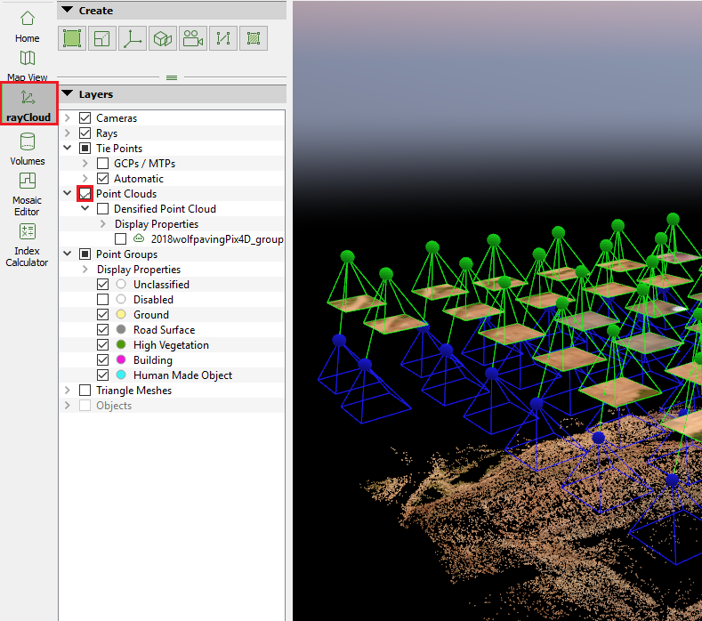 |
| Figure 2: Activating Point Clouds in Pix4D |
Step 2:
Once complete, uncheck Cameras and Tie Points as shown in figure 3 to be able to view the point cloud better.
 |
| Figure 10: Locating the Hillshade Tool |
Step 3:
Move the map over to the area of interest by clicking and dragging it and/or zooming using the scroll wheel on the mouse as necessary to get it into frame. In our case, the area of interest, shown in figure 4, was several stockpiles located in the north corner of the point cloud.
 |
| Figure 4: Stockpile Location |
Once there, inspect the area by holding down the scroll wheel to orbit the area to get a good understanding of what will be analyzed using volumetric analysis.
Step 4:
To calculate the volume of a specific area of interest, click on Volumes in the sidebar and click on the New Volume tool
 then click around the perimeter of the area of interest making sure to error wide of the edge so that the measurement tool can gain an accurate base measurement to work with and accurately determine the volume above that base plane. *Note: When clicking, use the scroll wheel to orbit around the area of interest to help determine what should be included in it.
Once the area of interest is enclosed, right click to close the polygon then click the Compute button as shown in figure 5.
 |
| Figure 5: Computing the Volume of the Area of Interest |
After Pix4D calculates the volume, the values should be displayed where the Compute button was located.
*Note: One can rename the area of interest by clicking on ‘Volume 1’ and typing the desired name.
Step 5:
Once the volume is computed, one may copy the information displayed to a clipboard and paste it where desired, by clicking on the icon highlighted below in figure 6.
 |
| Figure 6: Copying to Clipboard |
How to Perform Volumetric Analysis Using ArcMap:
Step 1:
Open ArcMap and click on the Catalog tab on the right sidebar as shown in figure 7 then click on the folder connection icon
 .
. |
| Figure 7: Search and Catalog Tools Located in Right Sidebar |
Step 2:
Connect to the folder where the data from the project will be stored and click OK (see figure 8).
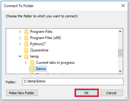 |
| Figure 8:Establishing a Folder Connection |
Step 3:
The next step in the process is to create a geodatabase for the project. A geodatabase is a smart folder containing all of the linked geographic information, attributes, tables, raster datasets and, feature classes created while working on a project. Geodatabases have a special information model to allow them to relate these various pieces of information together so they may be effectively used in the ESRI ArcGIS software.
In order to create a geodatabase, click on the Catalog tab on the right sidebar of the screen, right click on the folder created in step 2, click New then click File Geodatabase. Figure 9 is an image that shows how to create a geodatabase.
 |
| Figure 9: Creating a Geodatabase |
Step 4:
Click the Add Data icon
 located in the first row of icons at the top of the screen and add the DSM on which one wishes to perform Volumetric Analysis.
Step 5:
The next step in the process is to perform a hillshade operation to allow the user to more easily see changes in topography of the DSM.
To perform a hillshade operation, click on the Search tab on the right sidebar as shown in figure 7. Next, click on Tools, type “hillshade” into the search bar and, select the first tool in the list. Figure 10 shows how to locate the correct hillshade tool.
 |
| Figure 10: Locating the Hillshade Tool |
Once selected, a window labeled “hillshade” should appear. Within this window, in the Input raster box, select the down arrow and select the DSM. Next, click on the file icon next to the Output Raster box, double click on Folder Connections, find the folder where the geodatabase is located, click on it to highlight it, add a name that is less than 13 characters long at the bottom and click Save. Figure 11 shows the steps listed above in order from 1 to 5 and where to save the Output Raster hillshade once it is generated.
 |
| Figure 11: Output Raster Location |
Now that the input and output rasters have been taken care of, click OK at the bottom of the hillshade window to begin the processing.
Step 6:
Once complete, create a Feature Class by opening Catalog tab, right clicking on the geodatabase created in step 3, clicking on new and, clicking Feature Class. A Feature class is similar to a shapefile in that they both contain features and attribute data; however, a feature class allows the user to do more advanced operations than a shapefile would allow. See figure 12 below to see a visual representation on how to locate the Feature Class.
 |
| Figure 12: How to Add a Feature Class |
Once Feature Class is clicked, a window should appear labeled New Feature Class. Name the feature class and click Next at the bottom of the window.
On the next page, click on the down arrow next to the globe icon
 then click Import. A new window should appear labeled Browse for Datasets or Coordinate Systems. This window, as the name suggests, sets the coordinate system for the Feature Class to match those of the DSM. In order to do this, use the ‘Look in’ dropdown to locate the appropriate DSM and click Add as shown in figure 13.
 |
| Figure 13: Setting Data Coordinate System |
Once added, click next at the bottom of the New Feature Class window three times until the following window appears (see figure 14).
 |
| Figure 14: Adding Attribute Fields |
The above window is an attribute table that allows one to tie important information to the area, in this case a stockpile, so that when the data is viewed later on, the information about it will be linked and easily accessible.
To enter attribute information to this table, click on the first available spaces below the Field Name column, then add the following attribute data: Pile_ID, Volume_m^3 and, Base_Pile_Elevation. *Note: Feel free to add more fields as necessary to help describe different attributes of the area of interest.
Once Field Names have been added, in the Data Type column, use the drop down list to select the appropriate type of data for each of the Field Names. There are several options to choose from however for our dataset, set the Data Type as shown below in figure 15.
 |
| Figure 15: Setting the Type of Data |
Step 7:
Click on the Editor Toolbar
 located at the top of the screen in the first row of icons, then click the Editor dropdown as shown in figure 16 and click Start Editing.
 |
| Figure 16: Starting Editing |
Once Start Editing has been activating and the tools in the Editor Toolbar are no longer grayed out, click on the Create Features icon
 . when the menu appears on the right hand side of the screen, click on the feature that appears. Once selected, a Construction Tools menu should appear. Click on Polygon then click around the base of the feature, making sure to leave some room around the base so that the volumetrics tool can accurately determine the volume. When done tracing around the area, double click to create the last point and close the polygon then click Stop Editing. Figure 17 below shows the process of creating the polygon.
 |
Figure 17: Creating a Polygon |
Step 8:
The next step in the process is to use a tool called Extract by Mask. This tool takes a base raster and uses a mask to clip out an area of interest so that analysis can be performed on just that clipped-out portion. Figure 18 from ESRI’s ArcGIS for Desktop website, shows the process of using the Extract by Mask feature to perform specific localized analysis.
 |
| Figure 18: Applying the Extract by Mask Feature |
To perform the Extract by Mask, click on the Search tab, type in “extract by mask” and select Extract by Mask (Spatial Analyst). A window should appear with the corresponding tool. In the Input Raster box, select the down arrow and select the DSM. Next, click Input Raster or feature mask data and select the polygon file created in the previous step. For the Output Raster box, double click on Folder Connections, find the folder where the geodatabase is located, click to highlight it, add a name that is less than 13 characters long at the bottom, click Save then click OK to create the extraction. Figure 19 shows the steps listed above on how to perform an Extract by Mask.
 |
| Figure 19: Performing an Extract by Mask |
Step 9:
The next step is to take the clipped extraction and use the Surface Volume (3D Analyst) to calculate the volume of the the area of interest.
Before using this tool, one first has to know the base elevation of the area of interest. To do this, click on the information tool
 and when the Identify window pops up, set the Identify From drop down to the extraction created in step 8. Next, click around the base of the area of interest and record the base values.
Next, click on the Search tab, type in “surface volume” and select Surface Volume (3D Analyst). When the window opens, click on the down arrow and select the extraction created in step 8 for the Input Surface. Set the Output Text File, using the file icon, to the folder where the geodatabase for the project is kept and name the file. Next, set the Reference plane to ABOVE, set the Plane Height to the value gathered by the identify tool earlier and, click OK. *Note here that if one is performing the analysis with a concave surface, set the Plane Height to below so that it takes the volume below the plane rather than above. Figure 20 is an image of how to setup the Surface Volume tool.
 |
| Figure 20: Using the Surface Volume (3d Analyst) Tool |
In order to perform analysis comparing a multiple datasets of a location over time, one has to resample the data so that the pixel sizes from the datasets are the same. To do this using ArcMap, first follow all the steps above relating to ArcMap up to step 9.
Before using the Surface Volume tool, click on the Search tab and type in “resample” and click on the Resample (Data Management) tool. When the Resample window opens, use the drop down under Input Raster to select the extraction from the Extract by Mask step. For the Output Raster Dataset, use the folder icon to save it to the geodatabase. *Note: The next line, Output Cell Size can be used if one wishes to set one dataset to match another exactly. This will not be used in this case, because it is often better to sample to a standard cell size.
Just below Output Cell Size, there are two boxes where one can set a specific cell size for each pixel. The datasets that were worked with in this assignment were set to 0.1 by 0.1 (10cm by 10cm) cell size.
The Resampling Technique box allows the user to define which technique to use to combine cells and the correct one to use depends on the type of data being collected. For the purpose of this assignment, NEAREST was selected. *Note: If one clicks on Show Help>> at the bottom of the window, one can read about the different options and which option would be best for the data being resampled.
At the bottom of the Resample window, click OK. Figure 21 shows the resampling window with its options as described above.
 |
| Figure 21: Resampling Window in ArcMap |
Once the resampling is complete, one can perform the surface volume analysis as specified in step 9 of the Volumetric Analysis tutorial above.
Discussion/Results:
Using the methods shown above, two datasets were analyzed volumetrically using Pix4D and ArcMap. The two datasets used were Wolfpaving and Litchfield. The Wolfpaving dataset, of a mining operation, was used to calculate and compare the volume of three different stockpiles (Pile A, B and, C) using Pix4D versus using ArcMap. The second dataset of a Litchfield dredging operation was used to compare the volume of one pile over time.
Using Pix4D Versus ArcMap for Volumetric Analysis:
When performing volumetrics using Pix4D on Wolfpaving, the steps to follow were very simple and once the calculations were complete, the data could be copied to a clipboard for pasting into other programs. Figure 22 below shows Piles A, B and, C in relation to each other and table 1 below that shows the results from Pix4D’s calculations on these piles.
 |
| Figure 22: Pile’s A, B, and, C Relative Size and Relative Location |
 |
| Table 1: Pix4D Volumetric Results for Pile A, B and C |
Once the volumetrics for Wolfpaving were calculated using Pix4D, they again were calculated using ArcMap and the above steps. The steps when using ArcMap were much longer and more complicated than the Pix4D results and once they were calculated, they were copied to a table and a map was created. Below is table 2 and figure 23 showing the results for the volumetric calculations using ArcMap.
Comparing the results from both Pix4D and ArcMap using the tables reveals that they are very different between the programs. These differences between the two programs could due to the method of calculation, differences in selection of the perimeter (Terrain Area) around the area of interest, or other reasons.
The Pix4D results from the Terrain Area compared to the Total Volume results seems smaller than it should be considering Terrain Area is a measure of a 2-dimensional area and the Total Volume is a measure of the 3-dimensional volume of the piles. One would expect the volume to be significantly larger than the area as shown by the ArcMap Calculations.
Using ArcMap for Temporal Volumetric Analysis:
After comparing the difference between using ArcMap and Pix4D for volumetric analysis, ArcMap was used to compare the volume of the Litchfield stockpile over time. This type if analysis is known as temporal analysis and is important if one wishes to track the progress of mining or dredging operations over time.
When performing temporal analysis it is important to have consistency between datasets. This can be achieved by flying with the same sensor at the same time of day, at the same altitude, etc between datasets so that as many variables other than the area of interest are minimized.
The Litchfield stockpile, shown in the figures below, was flown on multiple occasions and the stockpiles were extracted, resampled to 10cm GSD, and surface volume analyses were performed to compare the volumes over the dates shown in the figures below. Figures 24-26 are maps of the Litchfield stockpile from July 22nd through August 30th 2017.
Once volumetrics were performed on the Litchfield stockpile, a table (table 3) containing the plane height above which the surface volume was measured, the area of the pile on that plane and, the total volume of the pile on different dates was created.
 |
| Table 2: ArcMap Volumetric Results for Pile A, B and C |
 |
| Figure 23: ArcMap Wolfpaving Volumetric Results Map |
Comparing the results from both Pix4D and ArcMap using the tables reveals that they are very different between the programs. These differences between the two programs could due to the method of calculation, differences in selection of the perimeter (Terrain Area) around the area of interest, or other reasons.
The Pix4D results from the Terrain Area compared to the Total Volume results seems smaller than it should be considering Terrain Area is a measure of a 2-dimensional area and the Total Volume is a measure of the 3-dimensional volume of the piles. One would expect the volume to be significantly larger than the area as shown by the ArcMap Calculations.
Using ArcMap for Temporal Volumetric Analysis:
After comparing the difference between using ArcMap and Pix4D for volumetric analysis, ArcMap was used to compare the volume of the Litchfield stockpile over time. This type if analysis is known as temporal analysis and is important if one wishes to track the progress of mining or dredging operations over time.
When performing temporal analysis it is important to have consistency between datasets. This can be achieved by flying with the same sensor at the same time of day, at the same altitude, etc between datasets so that as many variables other than the area of interest are minimized.
The Litchfield stockpile, shown in the figures below, was flown on multiple occasions and the stockpiles were extracted, resampled to 10cm GSD, and surface volume analyses were performed to compare the volumes over the dates shown in the figures below. Figures 24-26 are maps of the Litchfield stockpile from July 22nd through August 30th 2017.
 |
| Figure 24: July 22nd Flight of Litchfield Stockpile Volumetric Map |
 |
| Figure 25: August 27th Flight of Litchfield Stockpile Volumetric Map |
 |
| Figure 26: August 30th Flight of Litchfield Stockpile Volumetric Map |
 | |
|
*Note: Looking at table 3 above, it is clear that the largest volume of material in the stockpile was around August 27th.
Volumetrics is a tool that many may find useful in certain applications such as mining and dredging. Using UAV systems to collect this data can be beneficial because a UAV system is able to gather higher resolution datasets with which to perform these volumetric analyses. With these systems and analysis methods it can allow companies to accurately determine quantities of material and thus they can determine overall costs and profits.
Final Note:
When comparing between the two methods of calculating volumetrics and which should be used, I would recommend using ArcMap as Professor Hupy has used its volumetrics to calculate the volume of piles at a mining operation and the measured values compared to the calculated values were within 0.01% of each other.
Conclusion:
Volumetrics is a tool that many may find useful in certain applications such as mining and dredging. Using UAV systems to collect this data can be beneficial because a UAV system is able to gather higher resolution datasets with which to perform these volumetric analyses. With these systems and analysis methods it can allow companies to accurately determine quantities of material and thus they can determine overall costs and profits.
Final Note:
When comparing between the two methods of calculating volumetrics and which should be used, I would recommend using ArcMap as Professor Hupy has used its volumetrics to calculate the volume of piles at a mining operation and the measured values compared to the calculated values were within 0.01% of each other.